Magnetic control demand analysis
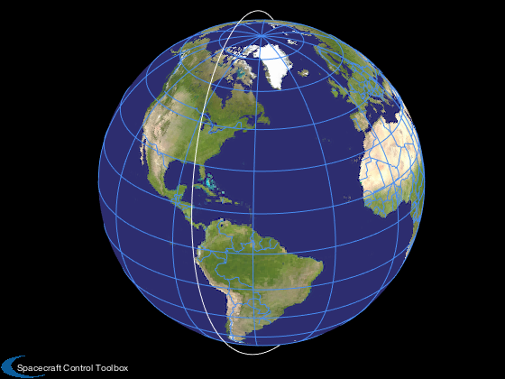
Put a satellite aligned with LVLH (nadir-pointing) in a 350 km inclined orbit and evaluate the ability of the magnetic control to create a particular torque along the orbit. There are 3 orthogonal torquers. Note that the pure x torque can only be created at certain points along the orbit.
-------------------------------------------------------------------------
Contents
%--------------------------------------------------------------------------
%   Copyright (c) 2011-2012 Princeton Satellite Systems, Inc.
%   All rights reserved.
%   Since version 10.
%--------------------------------------------------------------------------
Set up orbit and torquer model
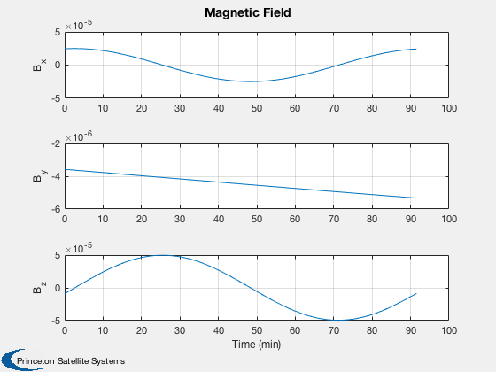
% Three orthogonal torquers
u = eye(3);

% Define the orbit
jD0       = Date2JD([2014 6 1 0 0 0]);
el        = [6378+350,0.9*pi/2,0,0,0,0];
[r, v, t]	= RVFromKepler( el );
n         = size(r,2);
PlotOrbit(r,t,jD0);

% Point the satellite along nadir
q = QLVLH( r, v );

% Compute the B field using a simple dipole model
jD  = jD0 + t/86400;
b   = QForm( q, BDipole( r, jD ) );

% Specify an x-axis torque demand
tDemand = 1e-5*[1;0;0]; % Nm
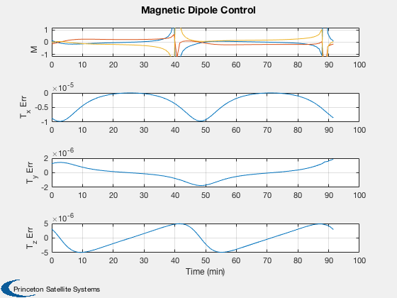
Evaluate the magnetic control demand
m     = zeros(3,n);
tErr  = zeros(3,n);
gamma = zeros(3,n);
for k = 1:n
  [m(:,k), tErr(:,k)] = MagneticControl( b(:,k), tDemand, u, 10 );
  gamma(:,k) = Mag(Cross(u,b(:,k)))';
end
[t, tL] = TimeLabl( t );
yL      = {'M','T_x Err' 'T_y Err' 'T_z Err'};
Plot2D( t, [m;tErr], tL, yL, 'Magnetic Dipole Control','lin',{[1 2 3],4,5,6});
subplot(4,1,1);
y = axis;
axis([y(1:2) -1.2 1.2])
yL      = {'B_x' 'B_y' 'B_z'};
Plot2D( t, b, tL, yL, 'Magnetic Field');

fprintf(1,'Average error = %12.4e Nm\n',mean(tErr,2));


%--------------------------------------
% PSS internal file version information
%--------------------------------------
Average error =  -3.3186e-06 Nm
Average error =  -2.1284e-10 Nm
Average error =   2.6316e-08 Nm