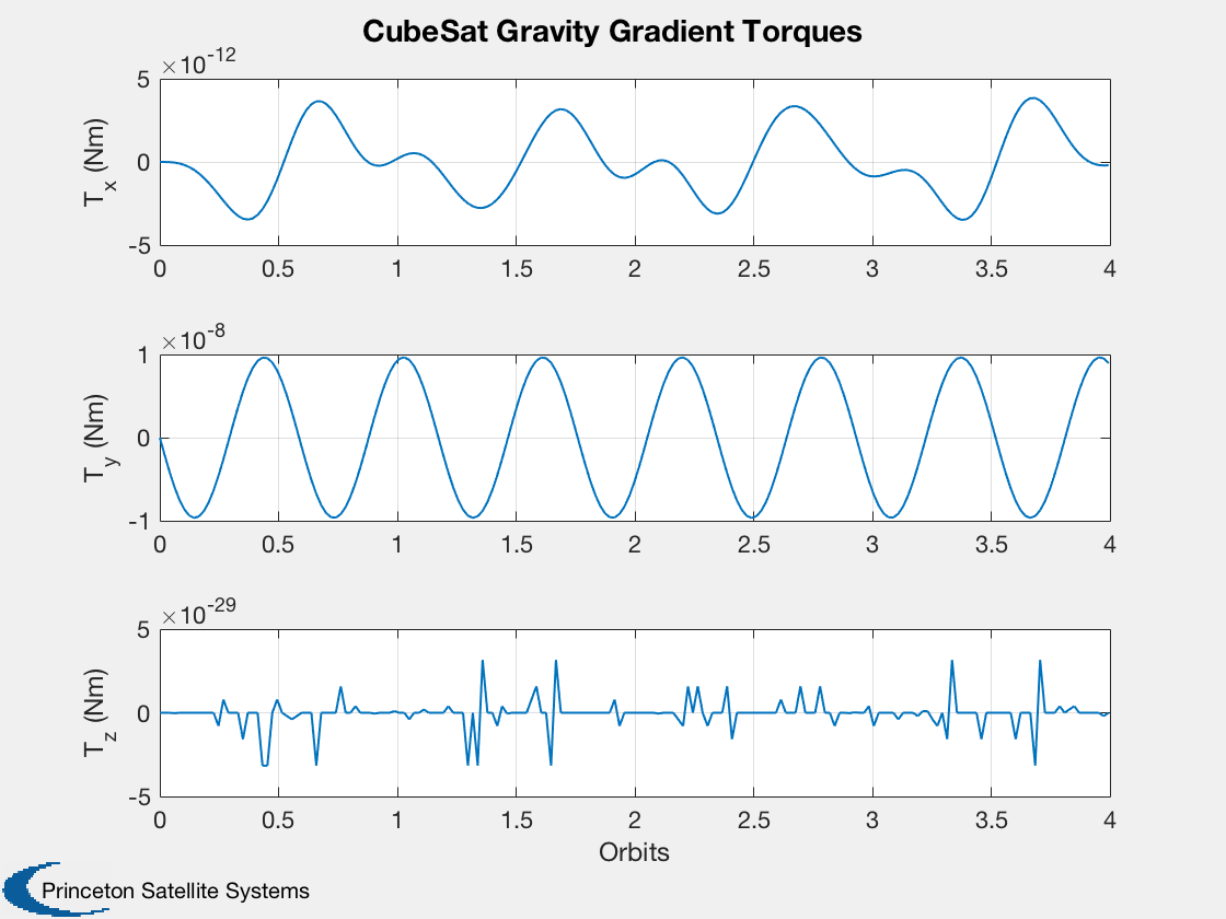
Demonstrate a CubeSat with gravity gradient stabilization.

The gravity gradient boom is along the Z axis in the body frame, and
produces restoring torques around X and Y.
----------------------------------------------------------------------
See also AnimQ, QForm, Plot2D, TimeLabl, RK4, Skew, Date2JD,
RHSCubeSat, BDipole
------------------------------------------------------------------------

Contents

%------------------------------------------------------------------------
%   Copyright (c) 2009 Princeton Satellite Systems, Inc.
%   All rights reserved.
%------------------------------------------------------------------------
%   Since version 10.
%  2016.0.1 - Fix velocity calulation to use VOrbit since mu is no longer in
%  RHS structure
%  2017.1 - Fix mass properties calculation to use AddMass
%------------------------------------------------------------------------

CubeSat model

%-------------
model = '1U';

Start with defaults for the RHS

%---------------------------------
d    = RHSCubeSat;

Initial state vector for a circular orbit

%------------------------------------------
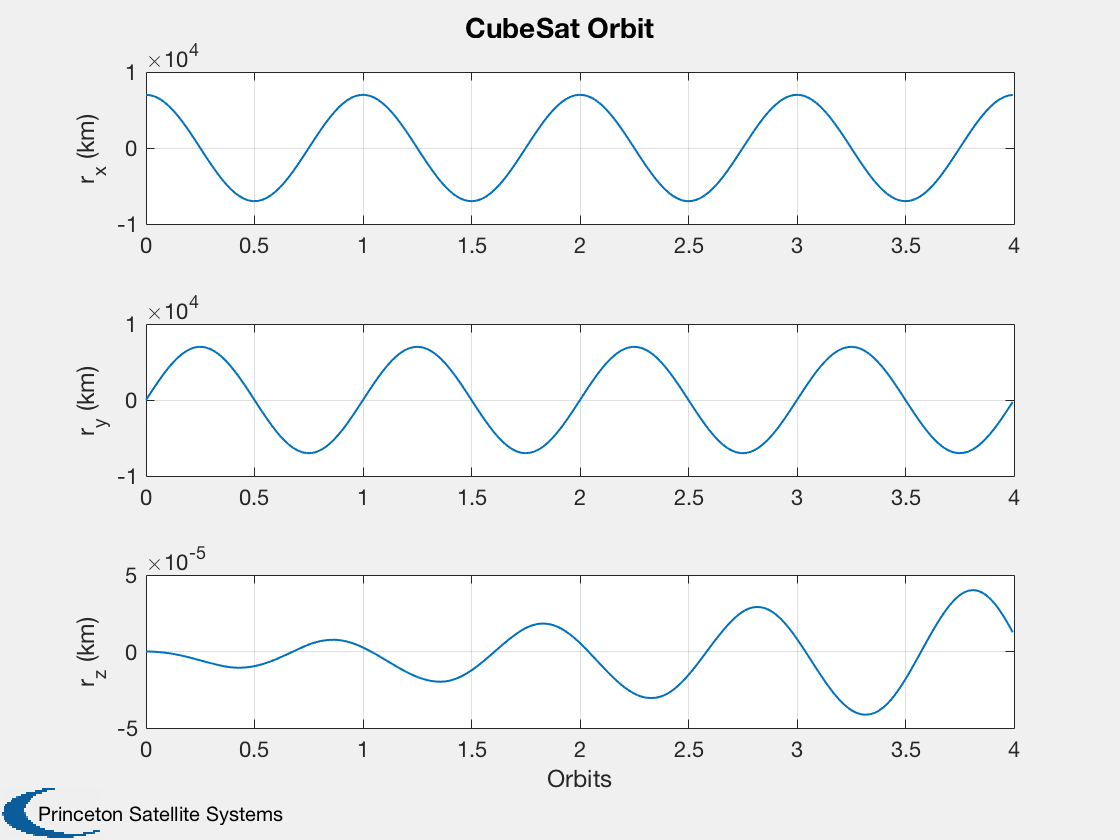
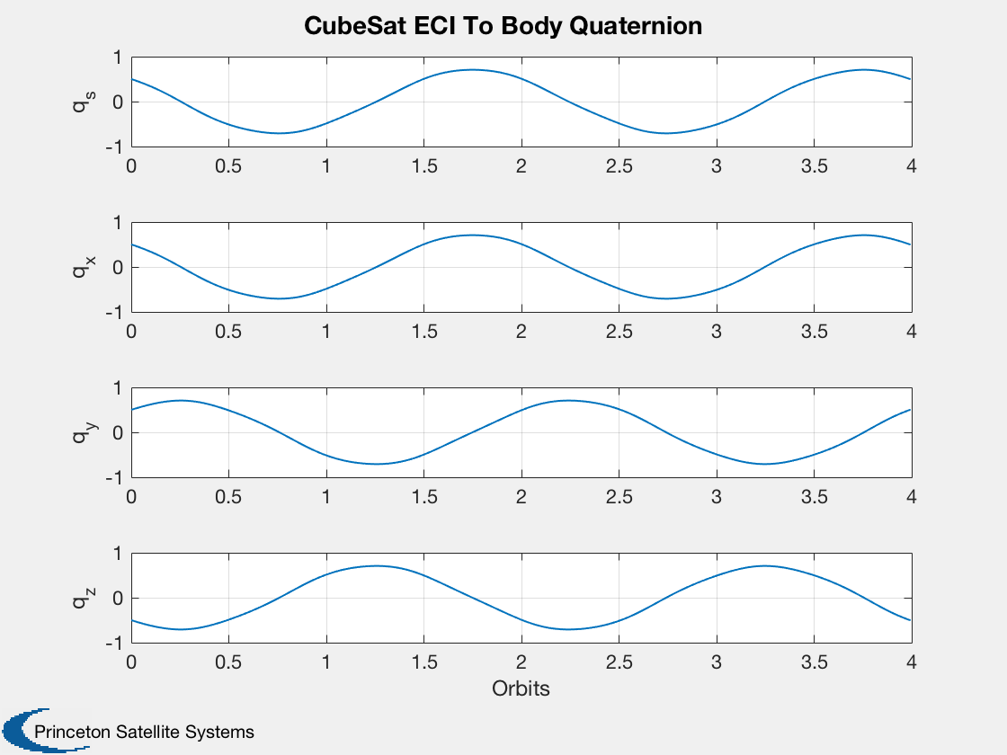
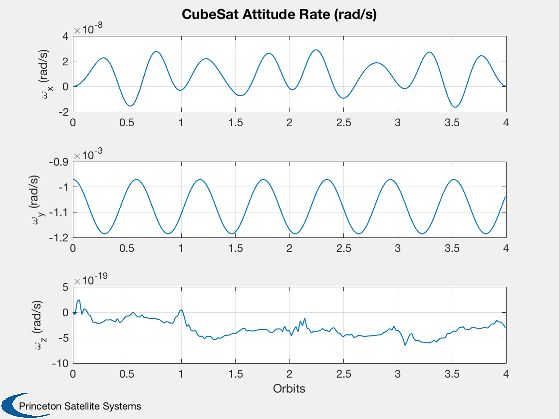
a    = 7000; % km
v    = VOrbit(a);
pOrb = Period(a);

% State is [position;velocity;quaternion;angular velocity; battery charge]
% CubeSats are about 1 kg per U
%-------------------------------------------------------------------------
r0 = [a;0;0];
v0 = [0;v;0];
q  = QLVLH( r0, v0 );
% Orbit rate is what we expect in the stable system. Introduce some offset
% to reveal the libration frequency.
w  = [0;-0.9*OrbRate(a);0];
b  = 0;
x  = [r0; v0; q; w; b];

Start Julian date

%------------------
d.jD0  = Date2JD([2012 4 5 0 0 0]);
d.rP   = 6378.165;

% Mass properties
%----------------
% The true inertia will be somewhat assymmetric. Always start with a
% symmetric inertia for code testing. Try switching between the simplified
% and true inertias.
% For modeling the gravity gradient boom, put a mass of 0.1 kg 50 cm from
% the CM of the spacecraft.
mSat = 0.85;
Isat = InertiaCubeSat( model, mSat );
rCM  = [0;0;0];
sat  = MassStructure(mSat, Isat, [0;0;0] );
mGG  = 0.1;
rGG  = [0;0;0.5];
Iboom = -mGG*SkewSq( rGG ); % point mass inertia
boom  = MassStructure(mGG, Iboom, rGG );
mass = AddMass( [sat boom] );
d.inertia = mass.inertia;
%d.inertia = diag([0.03 0.03 0.001]); % symmetric
d.mass = mass.mass;
s = LibrationFrequency( d.inertia, OrbRate(a) );
% Libration frequencies are around 1.7-2X orbit rate

Remove aero model.

The drag is very small at this altitude and the simulation is much faster without these calculations.

%-------------------
d.aeroData = [];

Add power system model

%-----------------------
d.power.solarCellNormal    = [1 -1;0 0;0 0];
d.power.solarCellEff       = 0.15;
d.power.effPowerConversion = 0.8;
d.power.solarCellArea      = 0.1*0.05*[1 1];
d.power.consumption        = 0.5;
d.power.batteryCapacity    = 100;

Initialize control

%-------------------
d.dipole = [0;0;0];

Simulation duration

%--------------------
orbits = 4;
tEnd   = pOrb*orbits;

Time step

%----------
dT    = 120;
nSim  = floor(tEnd/dT);

Initialize the plotting aray to save time

%------------------------------------------
xPlot = [x zeros(14,nSim)];
[xT, distur, tGG] = RHSCubeSat( x, 0, d );
dragPlot  = [distur.fAerodyn zeros(3,nSim)];
tAeroPlot = [distur.tAerodyn zeros(3,nSim)];
tMagPlot  = [distur.tMag zeros(3,nSim)];
tGGPlot   = [distur.tGG zeros(3,nSim)];
qLPlot    = zeros(4,nSim);

Run the simulation

%-------------------
t = 0;
h = waitbar(0,'CubeSat Simulation');
for k = 1:nSim

    % Magnetic field - the magnetometer output is proportional to this
    %-----------------------------------------------------------------
    bField = QForm( x(7:10), BDipole( x(1:3), d.jD0+t/86400 ) );

    % Control system placeholder
    %---------------------------
    % dipole from air-core torquers
    d.dipole = [0.0;0;0]; % Amp-turns m^2

    % A time step with 4th order Runge-Kutta
    %---------------------------------------
    x = RK4( @RHSCubeSat, x, dT, t, d );

    % Obtain effect of drag and control
    %----------------------------------
    [xT, dist] = RHSCubeSat( x, t, d );
    dragPlot(:,k+1) = dist.fAerodyn;
    tAeroPlot(:,k+1) = dist.tAerodyn;
    tMagPlot(:,k+1) = dist.tMag;
    tGGPlot(:,k+1) = dist.tGG;

    % Update plotting and time
    %-------------------------
    qLVLHToBody = QMult( QPose(QLVLH(x(1:3),x(4:6))), x(7:10) );
    qLPlot(:,k) = qLVLHToBody;
    xPlot(:,k+1) = x;
    t            = t + dT;

    waitbar(k/nSim,h);
end
close(h);

Plotting

%---------
t = (0:nSim)*dT;

Y-axis labels

%--------------
yL = {'r_x (km)' 'r_y (km)' 'r_z (km)' 'v_x (km/s)' 'v_y (km/s)' 'v_z (km/s)'...
      'q_s' 'q_x' 'q_y' 'q_z' '\omega_x (rad/s)' '\omega_y (rad/s)' '\omega_z (rad/s)' 'b (J)'};

Plotting

%----------
Plot2D( t/pOrb, xPlot( 1: 3,:), 'Orbits', yL( 1: 3), 'CubeSat Orbit' );
Plot2D( t/pOrb, xPlot( 7:10,:), 'Orbits', yL( 7:10), 'CubeSat ECI To Body Quaternion' );
Plot2D( t/pOrb, xPlot(11:13,:), 'Orbits', yL(11:13), 'CubeSat Attitude Rate (rad/s)' );
Plot2D( t/pOrb, tGGPlot,     'Orbits',  {'T_x (Nm)','T_y (Nm)','T_z (Nm)'},'CubeSat Gravity Gradient Torques')

% We aren't interested in these at the moment but keep them available
%Plot2D( t/pOrb, xPlot(   14,:), 'Orbits',  yL{14},     'CubeSat Battery' );
%Plot2D( t/pOrb, tMagPlot,    'Orbits',  {'T_x (Nm)','T_y (Nm)','T_z (Nm)'},'CubeSat Magnetic Torques')

AnimQ( qLPlot );


%--------------------------------------
% PSS internal file version information
%--------------------------------------

Published with MATLAB® R2016b