Demonstrate CubeSat attitude and power dynamics with reaction wheels.

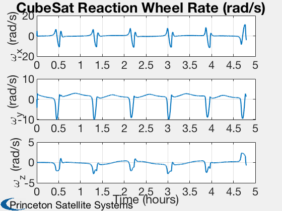
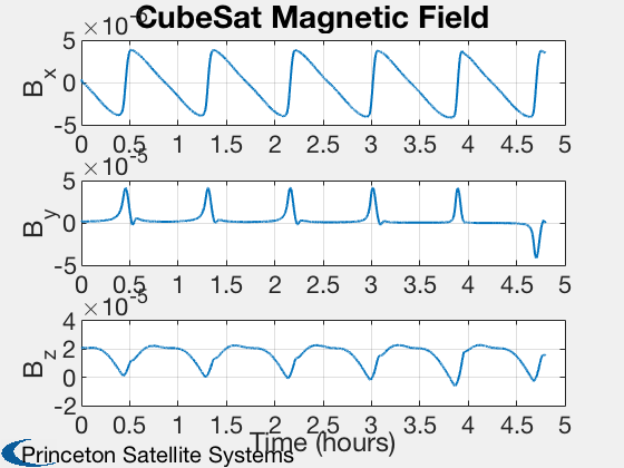
The model includes 3 orthogonal reaction wheels. The satellite is intialized into a polar orbit. The control law keeps the satellite aligned with the magnetic field, which results in flips at the poles.

------------------------------------------------------------------------- See also PIDMIMO, QForm, QTForm, CreateLatexTable, LatexScientificNotation, SaveStructure, Plot2D, TimeLabl, Dot, RK4, Unit, Date2JD, InertiaCubeSat, RHSCubeSat, BDipole, PID3Axis -------------------------------------------------------------------------

Contents

%------------------------------------------------------------------------
%   Copyright (c) 2009-2010,2016 Princeton Satellite Systems, Inc.
%   All rights reserved.
%------------------------------------------------------------------------
%   Since version 9 (2010).
%   2016.1 Add display of solar area with DrawCubeSatSolarAreas.
%------------------------------------------------------------------------

clear g; clear u; clear p; clear d;

Constants

%-----------
radToDeg        = 180/pi;
densitySilicon  = 2600;
densityAl       = 2700; % Aluminum
densityTungsten = 19300;

Simulation parameters

%-----------------------
days  = 0.2;
tEnd  = days*86400;
dT    = 1;
nSim  = ceil(tEnd/dT);

CubeSat model

Initialize data structure

%--------------------------
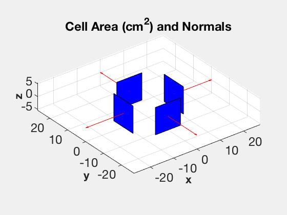
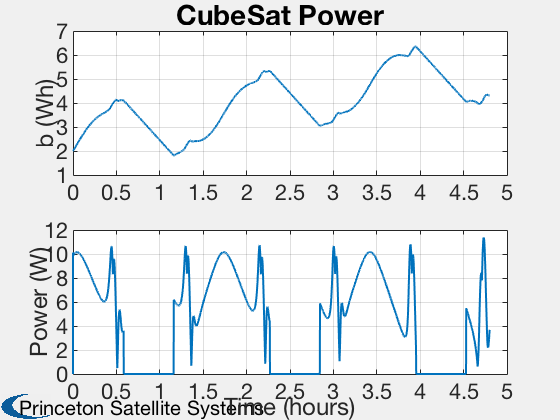
d = RHSCubeSat;

% CubeSats are 1 kg per U
%---------------
model = '3U';
[area,nFace,rFace] = CubeSatFaces( model, 1 );
d.mass = 3; % kg
d.inertia = InertiaCubeSat( model, d.mass );

% Model data
%------------
d.surfData.area = area;
d.surfData.nFace = nFace;
d.surfData.rFace = rFace;
d.surfData.att.type = 'eci';

% Reaction wheel design
%-----------------------
d.kWheels    = 14:16; % indices of wheel states
radius       = 0.020;
thickness    = 0.004; % This is 4 mm
volRWA       = pi*radius^2*thickness;
massRWA      = volRWA*densityTungsten; % Mass from density x volume
d.inertiaRWA = (massRWA/2)*radius^2; % Polar inertia
thicknessSolarPanel = 0.004;

% Add power system model
% Lithium batteries are 360000 J/kg according to
% http://en.wikipedia.org/wiki/Lithium-ion_battery,
% so size the battery for 100 g = 36000 J = 10 Wh
% Solar cell efficieny is 27% to 29.5% according to Emcore,
% http://www.emcore.com/solar_photovoltaics/
%---------------------------------------------------------
d.power.solarCellNormal    = [1 1 -1 -1 0 0 0 0;0 0 0 0 1 1 -1 -1;0 0 0 0 0 0 0 0];
d.power.solarCellEff       = 0.295;
d.power.effPowerConversion = 0.9;
d.power.solarCellArea      = 0.1*0.116*ones(1,8);
d.power.consumption        = 4;
d.power.batteryCapacity    = 36000;
volSolarPanel              = d.power.solarCellArea(1,1)*thicknessSolarPanel;
massSolarPanel             = volSolarPanel *densitySilicon;
DrawCubeSatSolarAreas(d.power)

ans = 
  Figure (PlotPSS) with properties:

      Number: 1
        Name: 'DrawCubeSatSolarAreas'
       Color: [0.94 0.94 0.94]
    Position: [440 378 560 420]
       Units: 'pixels'

  Use GET to show all properties

Initial state vector for a circular orbit

%------------------------------------------
x    = 6387.165+800; % km
v    = VOrbit(x);

r    = [x;0;0];                 % Position vector
v    = [0;0;v];                 % Velocity vector - polar orbit
q    = [1;0;0;0];               % Quaternion
w    = [0;0;0];                 % Angular rate of spacecraft
c    = [0;0;0];                 % Reaction wheel rates
b    = 2*3600;                  % Battery state of charge (J = Wh*3600)

% State is [position;velocity;quaternion;angular velocity;wheels;battery charge]
%-------------------------------------------------------------------------
x    = [r;v;q;w;c;b];

Start Julian date

%------------------
d.jD0  = Date2JD([2012 4 5 0 0 0]);

Design the PID Controller

Specify the z body axis for alignment with the chosen ECI vector

%-----------------------------------------------------------------
p                    = PID3Axis;
[p.a, p.b, p.c, p.d] = PIDMIMO( 1, 1, 0.01, 200, 0.1, dT );

p.inertia            = d.inertia;
p.max_angle          = 0.01;
p.accel_sat          = [100;100;100];
p.mode               = 1;
p.q_target_last      = q;
p.q_desired_state    = [0;0;0;1];
p.body_vector        = [0;0;1];

Atmosphere model data

Skip the J70 model as it is slow; use the commented out code to switch back if desired. AtmDens2 will be used instead.

d.atm = [];
% [aP, f, fHat, fHat400] = SolarFluxPrediction( d.jD0, 'nominal' );
% d.atm.aP      = aP(1);
% d.atm.f       = f(1);
% d.atm.fHat    = fHat(1);
% d.atm.fHat400 = fHat400(1);

Initialize the plotting array to save time

%--------------------------------------------
qECIToBody   = x(7:10);
bField       = QForm( qECIToBody, BDipole( x(1:3), d.jD0 ) );
p.eci_vector = Unit(bField);
angleError   = acos(Dot(p.eci_vector,QTForm(qECIToBody,p.body_vector)))*radToDeg;

xPlot        = [[x;0;0;0;0;angleError;bField;0;0;0] zeros(length(x)+11,nSim)];

Initialize the time display

%----------------------------
TimeDisplay( 'initialize', 'CubeSat RWA Sim', nSim );

Run the simulation

%-------------------
t = 0;

for k = 1:nSim
  % Display the status message
  %---------------------------
  TimeDisplay('update');

  % Quaternion
  %-----------
  qECIToBody   = x(7:10);

  % Magnetic field - the magnetometer output is proportional to this
  %-----------------------------------------------------------------
  bField       = QForm( qECIToBody, BDipole( x(1:3), d.jD0+t/86400 ) );

  % Control system momentum management
  %-----------------------------------
  d.dipole     = [0.0;0;0]; % Amp-turns m^2

  % Reaction wheel control - align with the magnetic field
  %-------------------------------------------------------
  p.eci_vector = Unit(bField);
  angleError   = acos(Dot(p.eci_vector,QTForm(qECIToBody,p.body_vector)))*radToDeg;
  [torque, p]  = PID3Axis( qECIToBody, p );
  d.tRWA       = -torque;

  % A time step with 4th order Runge-Kutta
  %---------------------------------------
  x            = RK4( @RHSCubeSat, x, dT, t, d );

  % Get the power
  %--------------
  [xDot, dist, power] = RHSCubeSat( x, t, d );

  % Update plotting and time
  %-------------------------
  hRWA         = x(14:16)*d.inertiaRWA;
  xPlot(:,k+1) = [x;power;torque;angleError;bField;hRWA];
  t            = t + dT;

end
TimeDisplay( 'close' );

Plotting

%---------
kP = 1:k+1;
[t, tL] = TimeLabl( (0:k)*dT );

Y-axis labels

%--------------
yL = {'r_x (km)' 'r_y (km)' 'r_z (km)' 'v_x (km/s)' 'v_y (km/s)' 'v_z (km/s)'...
      'q_s' 'q_x' 'q_y' 'q_z' '\omega_x (rad/s)' '\omega_y (rad/s)' '\omega_z (rad/s)' ...
      '\omega_x (rad/s)' '\omega_y (rad/s)' '\omega_z (rad/s)' 'b (Wh)' 'Power (W)' ...
      'T_x (Nm)' 'T_y (Nm)' 'T_z (Nm)' 'Angle Error (deg)' 'B_x' 'B_y' 'B_z',...
      'H_x (Nms)' 'H_y (Nms)' 'H_z (Nms)'};

Plotting utility

%-----------------
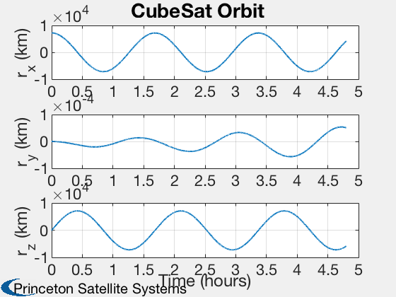
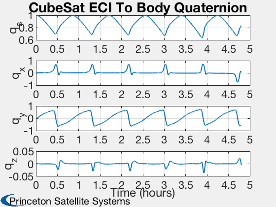
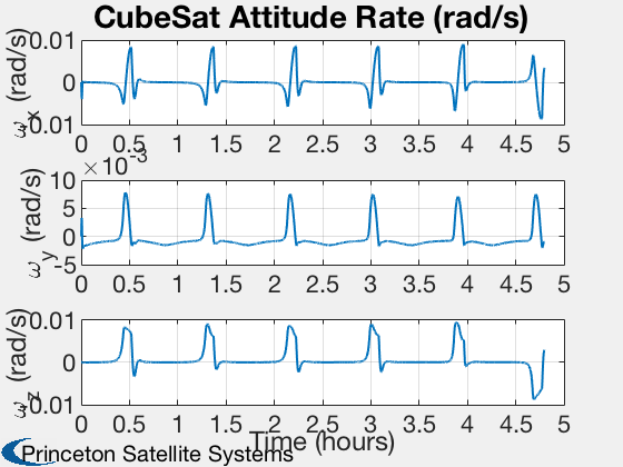
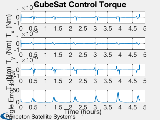
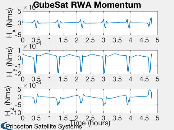
Plot2D( t, xPlot( 1: 3,kP), tL, yL(  1: 3), 'CubeSat Orbit' );
Plot2D( t, xPlot( 7:10,kP), tL, yL(  7:10), 'CubeSat ECI To Body Quaternion' );
Plot2D( t, xPlot(11:13,kP), tL, yL( 11:13), 'CubeSat Attitude Rate (rad/s)' );
Plot2D( t, xPlot(14:16,kP), tL, yL( 14:16), 'CubeSat Reaction Wheel Rate (rad/s)' );
Plot2D( t, [xPlot(17,kP)/3600;xPlot(18,kP)], tL, yL( 17:18), 'CubeSat Power' );
Plot2D( t, xPlot(19:22,kP), tL, yL( 19:22), 'CubeSat Control Torque' );
Plot2D( t, xPlot(23:25,kP), tL, yL( 23:25), 'CubeSat Magnetic Field' );
Plot2D( t, xPlot(26:28,kP), tL, yL( 26:28), 'CubeSat RWA Momentum' );

maximumTorque   = max(max(abs(xPlot(19:21,kP))));
maximumMomentum = max(max(abs(xPlot(26:28,kP))));
maximumSpeed    = max(max(abs(xPlot(14:16,kP))));

Create a table of output

%--------------------------
g{1,1} = 'Reaction Wheel Inertia';
g{1,2} =  LatexScientificNotation( d.inertiaRWA, 1);
g{1,3} = 'kg-m$^2$';

g{2,1} = 'Reaction Wheel Radius';
g{2,2} =  sprintf('%8.4f',radius*1000);
g{2,3} = 'mm';

g{3,1} = 'Reaction Wheel Thickness';
g{3,2} =  sprintf('%8.4f',thickness*1000);
g{3,3} = 'mm';

g{4,1} = 'Maximum RWA torque';
g{4,2} =  LatexScientificNotation( maximumTorque, 4);
g{4,3} = 'Nm';

g{5,1} = 'Maximum RWA Momentum';
g{5,2} =  LatexScientificNotation( maximumMomentum, 4 );
g{5,3} = 'Nms';

g{6,1} = 'Maximum RWA Rate';
g{6,2} =  sprintf('%12.4f',maximumSpeed*30/pi);
g{6,3} = 'RPM';

g{7,1} = 'Solar Cell Efficiency';
g{7,2} =  sprintf('%8.4f',d.power.solarCellEff);
g{7,3} = '';

g{8,1} = 'Power Conversion Efficiency';
g{8,2} =  sprintf('%8.4f',d.power.effPowerConversion);
g{8,3} = '';

g{9,1} = 'Panel Area';
g{9,2} =  sprintf('%8.4f',d.power.solarCellArea(1)*1e4);
g{9,3} = 'cm$^2$';

g{10,1} = 'Average Power Consumption';
g{10,2} =  sprintf('%8.1f',d.power.consumption );
g{10,3} = 'W';

g{11,1} = 'Battery Capacity';
g{11,2} =  sprintf('%8.1f',d.power.batteryCapacity/3600);
g{11,3} = 'Wh';

CreateTable( g );

     Reaction Wheel Inertia -    1.9 $\times 10^{-5}$  - kg-m$^2$ 
      Reaction Wheel Radius -                 20.0000  -       mm 
   Reaction Wheel Thickness -                  4.0000  -       mm 
         Maximum RWA torque - 7.1802 $\times 10^{-6}$  -       Nm 
       Maximum RWA Momentum - 2.2400 $\times 10^{-4}$  -      Nms 
           Maximum RWA Rate -                110.2463  -      RPM 
      Solar Cell Efficiency -                  0.2950  -          
Power Conversion Efficiency -                  0.9000  -          
                 Panel Area -                116.0000  -   cm$^2$ 
  Average Power Consumption -                     4.0  -        W 
           Battery Capacity -                    10.0  -       Wh 

Save data for the budgets

%--------------------------
u.rwa.mass          = massRWA;
u.rwa.volume        = volRWA;
u.solarPanel.mass   = massSolarPanel;
u.solarPanel.volume = volSolarPanel;

SaveStructure(u,'BudgetData.mat');


%--------------------------------------
% PSS internal file version information
%--------------------------------------

Published with MATLAB® R2016b